Example: An adjacency matrix
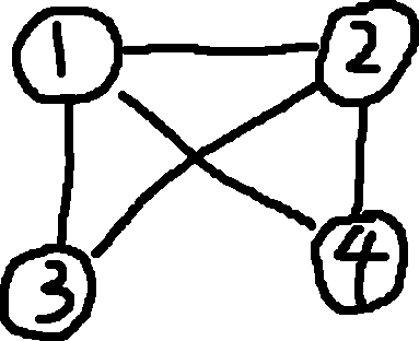
| 1 | 2 | 3 | 4 | |
|---|---|---|---|---|
| 1 | 0 | 1 | 1 | 1 |
| 2 | 1 | 0 | 1 | 1 |
| 3 | 1 | 1 | 0 | 0 |
| 4 | 1 | 1 | 0 | 0 |
There are two parameters to represent, vertices and edges.
\text{Graph: } G = (V, E)
There are two methods of representation (mathematically):
List all vertices.
Note — Properties:
- Total Size: \Theta ( |V| + |E| )
- Better on sparse graphs11. Graphs where |E| is much closer to |V| than to |V|^2.
| Node | Adjacency List |
|---|---|
| 1 | \to 2 \to 3 \to 4 |
| 2 | \to 1 \to 3 \to 4 |
| 3 | \to 1 \to 2 |
| 4 | \to 1 \to 2 |
NTS: Remember 2 connects to 4, 3 doesn’t connect to 4.
Store vertices in a square matrix
Note — Properties:
- Total Size: \Theta( |V|^2 )
- Better on dense graphs22. Graphs where |E| is close to |V|^2..
| 1 | 2 | 3 | 4 | |
|---|---|---|---|---|
| 1 | 0 | 1 | 1 | 1 |
| 2 | 1 | 0 | 1 | 1 |
| 3 | 1 | 1 | 0 | 0 |
| 4 | 1 | 1 | 0 | 0 |
Graph Traversal: Problem of visiting all nodes in a graph in a particular manner, updating/checking values along the way.
There are two elementary traversal strategies using brute-force algorithms:
Note — Both provide efficient ways to visit each vertex and edge, they only differ in order of visiting.
Visit vertices by always moving away from the last-visited vertex to an unvisited one. Backtracks if no adjacent unvisited vertex is available.
Note — Data Structure: Stack (FILO)
- Vertex pushed on when it’s reached for the first time.
- Vertex popped off when it becomes a dead end33. i.e., no adjacent unvisited vertex..
Consider a graph with vertices a, b, c, d, e, f where a connects to c and d, c connects to f and b, etc.
Mathematically, we could phrase this as:
a_{1, 6} c_{2, 5} d_{3, 1} f_{4, 4} b_{5, 3} e_{6, 2}
Note — First subscript is the order something was popped-on, second subscript is order it was popped-off.
We aren’t done though, there’s the other portion to traverse:
g_{1,4} h_{2,3} i_{3,2} j_{4,1}
Now, we are truly done.
ALGORITHM DFS(G)// Implements a depth-first search traversal of a given graph// Input: Graph G = <V, E>// Output: Graph G with its vertices marked with consecutive integers// in the order they're first encounteredmark each vertex in V with 0 as a mark of being "unvisited"count \leftarrow 0for each vertex v in V doif v is marked with 0dfs(v)ALGORITHM dfs(v)// visits recursively all the unvisited vertices connected to vcount \leftarrow count \text{$+$} 1; mark v with countfor each vertex w in V adjacent to v doif w is marked with 0dfs(w)
Analysis — Time complexity is \Theta(|V|^2) for adjacency matrix and \Theta(|V| + |E|) for adjacency list. Space complexity is O(|V|) for the recursion stack.
Note — You can use the traversal’s stack to construct a tree-like graph, which we’ll call a DFS forest.
DFS Forest:
Example: Graph to Stack to Forest
The traversal stack defines the parent-child relationships for the tree edges.
Constructing the DFS Forest from this stack, we get a tree where a connects to c, c connects to d and f, and back edges connect nodes to previously visited ancestors.
Note — For us, we’ll just look at the original graph to determine back-edges, as determining this from the traversal stack is a little more involved.
- We just use the traversal stack to build the easier tree edges.
Visit verticies by moving across to all neighbors of last-visited vertex.
Instead of plunging deep, we explore layer by layer, visiting all neighbors of a node before moving to the neighbors’ neighbors.
Note — Data Structure: Uses queue (FIFO)
More Notes:
ALGORITHM BFS(G)// Implements a breadth-first search traversal of a given graph// Input: Graph G = <V, E>// Output: Graph G with its vertices marked with consecutive integersmark each vertex in V with 0count \leftarrow 0for each vertex v in V doif v is marked with 0bfs(v)ALGORITHM bfs(v)// visits all the unvisited vertices connected to vcount \leftarrow count \text{$+$} 1; mark v with countinitialize a queue with vwhile the queue is not empty dofor each vertex w in V adjacent to the front vertex doif w is marked with 0count \leftarrow count \text{$+$} 1; mark w with countadd w to the queueremove the front vertex from the queue
Analysis — Time complexity is \Theta(|V|^2) for adjacency matrix and \Theta(|V| + |E|) for adjacency list. Space complexity is O(|V|) for the queue.
Note — You can use the traversal’s queue to construct a tree-like graph.
Similar to DFS, tree edges are formed when a node discovers an unvisited neighbor. Cross edges (instead of back edges) can connect nodes on the same or adjacent levels.